Analyzing A Decade's Worth Of My Movie Ratings

30 May 2022

---

As we have established, I have rated over a thousand movies on IMDb thus far. At the time of this writing, it’s a treasure trove of data over a decade in the making. I’ve had many ideas to find interesting patterns in it.

I decided to poke and prod at an exported copy. IMDb’s CSV export includes basic data about each title - the IMDb user rating, release date etc. To get the real juicy info, I had to cross-reference it with full IMDb datasets. I finally had an excuse to put my Rackfocus project to good use. It’s a little Python command line utility (install using pip install rackfocus) to pull freely available IMDb datasets and organize them into convenient SQLite tables.

Here are some interesting finds from my own ratings. If you too have a trove of ratings on IMDb and want to run these (and more) analyses yourself, skip to the end for instructions.

To set the stage, I rate every movie I watch. I generally don’t review them in writing. For the most part, I save a rating within hours of watching. Occasionally, I may forget for a couple of days. Very rarely, I may change a rating a few days after. On the rare occasion that I rewatch a movie, I will reconsider my rating. I have noticed that in the majority of those cases, even years later, my rating does not change.

IMDb ratings are on a scale from 1 to 10 (not 0 to 10).

I should disclaim that while I work at Amazon at the time of publishing this, I am not affiliated with IMDb.

“Favorite” Directors

For instance, I tried generating a data-driven list of my “favorite” directors. I first used a naïve method, simply adding up all my scores for all movies, grouped by director. Here’s what that looked like.

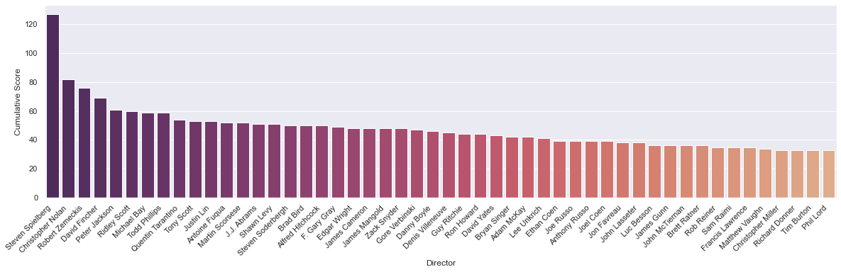
Turns out this is wildly skewed by people who have directed lots of movies.

I then decided to refine my method and find average ratings per director. In theory, this would get me a more meaningful list. Instead, it gave me a smattering of directors who have either directed very few movies that I’ve really enjoyed, or directors that I haven’t watched all that much, but really enjoyed nevertheless. Here are the top few from that list.

Rank	Director	Mean Rating
1	Dan Trachtenberg	10.000000
2	Lenny Abrahamson	10.000000
3	Jared Bush	10.000000
4	Ronnie Del Carmen	10.000000
5	Joss Whedon	10.000000
6	Nathan Greno	10.000000
7	Joe Russo	9.750000
8	Anthony Russo	9.750000
9	Jon Watts	9.666667
10	Rich Moore	9.333333
11	Byron Howard	9.333333
12	Josh Cooley	9.000000
13	Garth Davis	9.000000
14	Roger Allers	9.000000,
15	Daniel Scheinert	9.000000

In retrospect, the initial list turned out to be a slightly better representation of my taste in movies. It’s not perfect, but it does give a glimpse into the kinds of movies I’m likely to pick, in addition to my rating.

Through The Years

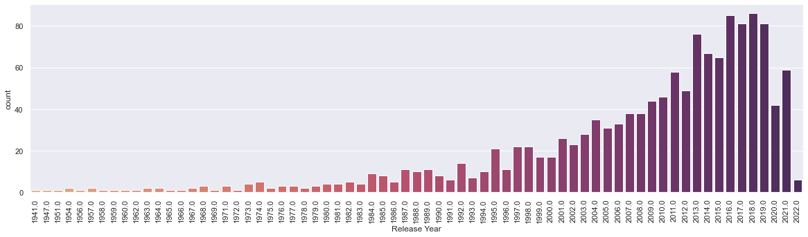
Here’s a histogram of the number of movies I’ve watched by release year.

To make any sense of this, I charted the number of movies released each year since the birth of cinema. It’s a simple plot consisting of all IMDb titles of type “movie”.

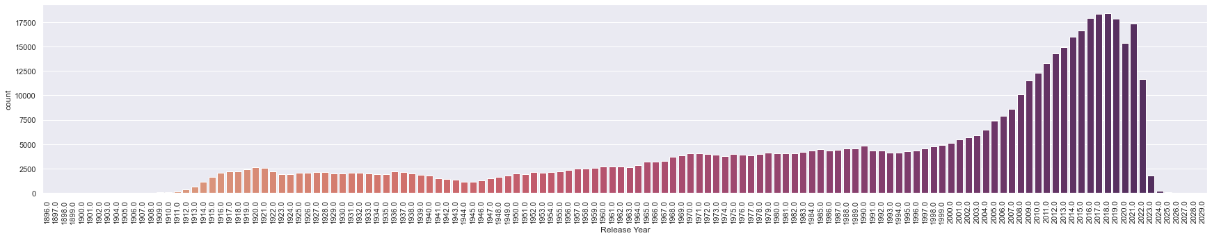
While the shapes of the two histograms match at first glance, I was surprised to see that I over-index so much in movies released this millenium.

Side-note: It’s also fascinating to see the unprecedented impact of the Covid-19 pandemic on release patterns. It will be interesting to plot this again in a few years.

A heatmap of my rating values against release year follows.

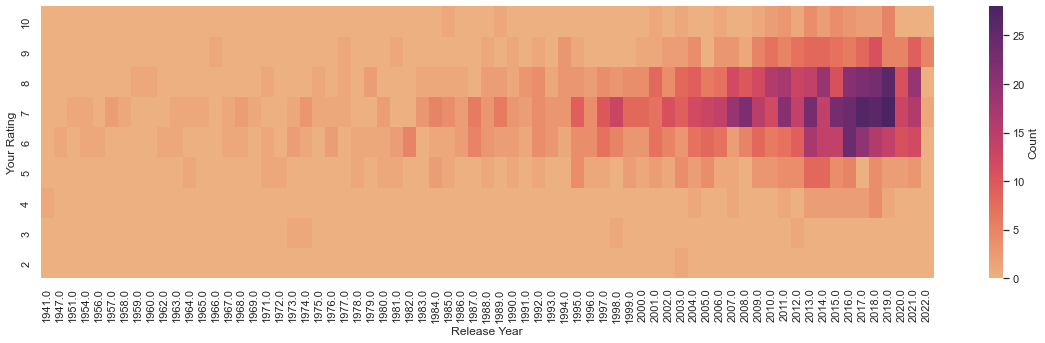
It would have been interesting to see more than one hot spot, especially if they were on different places on the y-axis. It would show any biases towards movies from specific eras. I’m glad to see that I don’t. There are some warm spots, however. At the risk of reading too much into it:

1. Just eyeballing the figure, I’ve watched slightly more movies released in 1997-98 than a few surrounding years. Honorable mentions from that year: Men in Black, The Game, Face/Off, Armageddon, The Big Lebowski, Rush Hour, Saving Private Ryan, Ronin, Money Talks, Mulan, and Good Will Hunting.
2. Year 2008 is also quite hot. Honorable mentions from that year: Cloverfield, Iron Man, The Dark Knight, Wanted, Sunshine Cleaning, Speed Racer, WALL·E, and Tropic Thunder.
3. Years 2010, 2011 and 2014 are highly rated. A handful of my top picks from that year, in no order: Inception, Toy Story 3, The King’s Speech, Unthinkable, Black Swan, Mission: Impossible - Ghost Protocol, Fast Five, Crazy, Stupid, Love, Super 8, The Adventures of Tintin, Chef, Captain America: The Winter Soldier, Gone Girl, The Guest, John Wick, and Edge of Tomorrow.
4. There is a bell curve around ratings 6-8 out of 10. This is analyzed further in the following section.

The Bell Curve

Let’s check how my ratings behave against normal distribution. Simplifying what the previous section’s heatmap shows by removing release years from the picture gets us this.

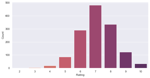
This shows low bias towards extremes. I’ve also maintained that this should be what any movie rating distribution should look like for two reasons.

1. It’s not u- or v-shaped. Bell curve resembles a normal distribution.
2. A shift to the right (as in, greater than 5 out of 10) is expected, as people watch movies not by random sampling, but based on what they know they’re likely to enjoy.

“Overrated” And “Underrated” Movies

I’ve been curious about this one for a long time. What are my biggest deviations from the IMDb crowd? I made two plots of extreme outliers - movies that I have absolutely loved, way more than the population, and ones that I’ve hated, and consider overrated.

We’re all aware of such outliers in our personal tastes. These are the conversation starters, the ones that incite debate and discord. And finally, I have data driven answers.

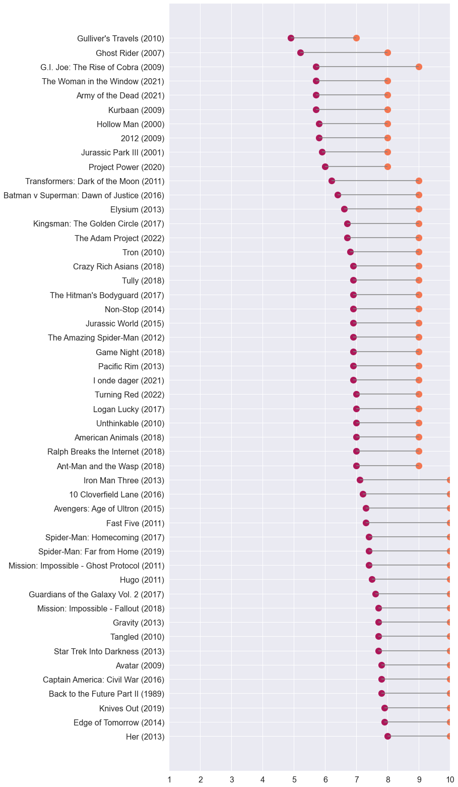
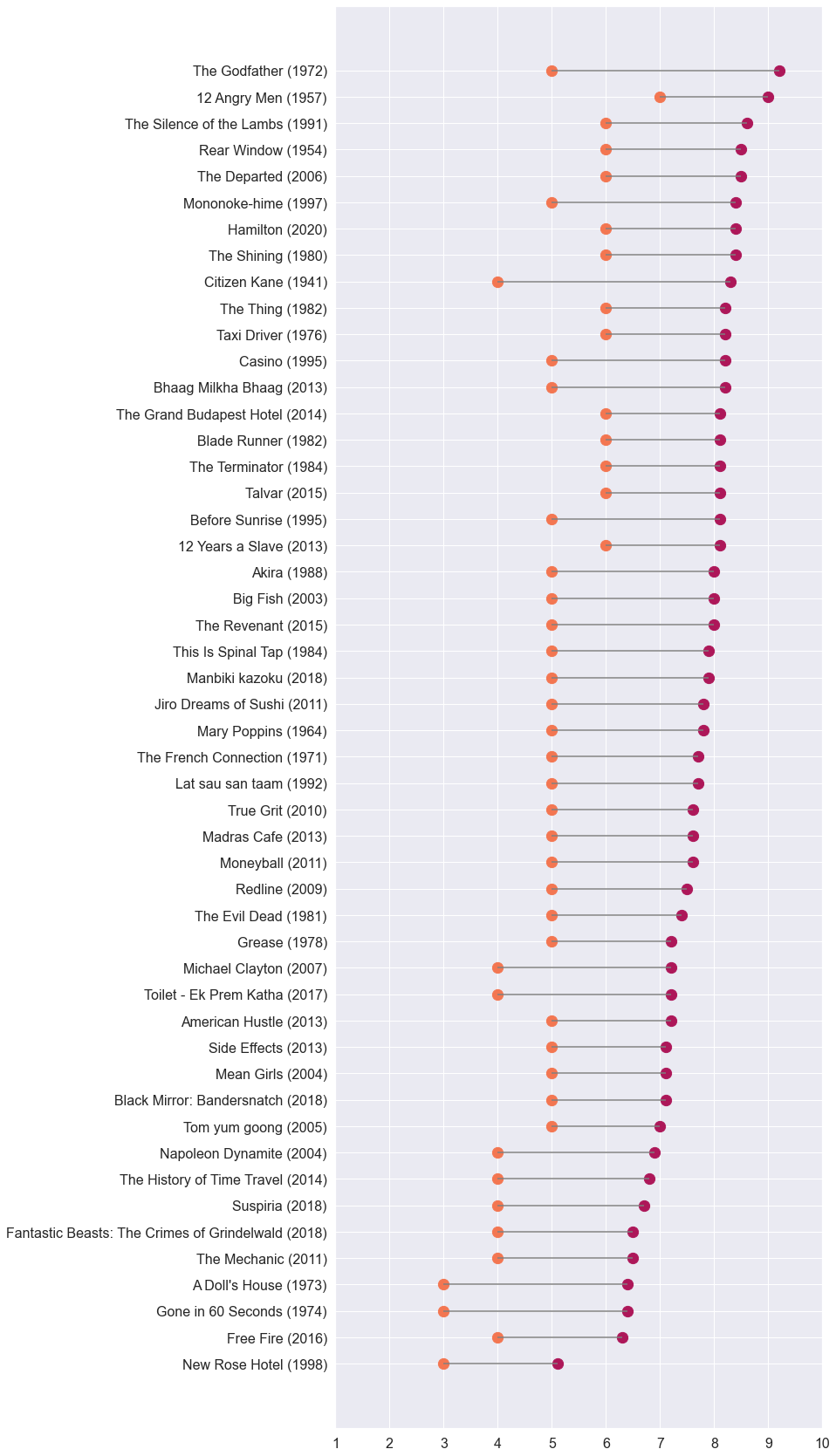
These lists comprise my 50 largest deltas anchored around IMDb averages on either end of the scale. The plots are sorted by IMDb ratings for easier visual skimming.

There are some titles that I knew would appear in these lists. I remember really liking G.I. Joe: The Rise of Cobra almost a decade ago, then being surprised by its IMDb rating. Lo and behold, it’s on my “underrated” list. Other titles, like Gulliver’s Travels, I blame on a less experienced teenage palette, or me being in a forgiving mood at the time. Except for these extremes, most movies on the “underrated” list appear to be titles received positively by fans, which I happened to rate 9 or 10 out of 10. As evident, I don’t hesitate to round up to 10 out of 10 ratings.

As for the “overrated” list, I was confident of two very well-regarded titles showing up - Citizen Kane and The Godfather - and they did. Napoleon Dynamite also appears in my top 50 “overrated” delta list. Now You See It on YouTube has a fascinating video essay on the hit-or-miss nature of this movie. Evidently, it missed me when I watched it.

All that said, these two lists are some of the extremes in my rating behavior. I watched many of these movies many years ago, and not more than once. It’s safe to assume that my ratings for these titles are the likeliest to change on rewatches.

Not Done Yet

Pretty interesting patterns so far, but I’m not done yet.

I hope to add more visualizations to my analysis notebook as I get more ideas.

One thing I wanted to check was my affinities towards studios and distributors. I know Marvel Studios and Pixar would likely top my preferences for studios. It would be interesting to see if I have any proclivities to rate releases from big distribution houses - Universal, 20th Century Studios, Lionsgate, etc. - higher or lower than others. Unfortunately, IMDb’s datasets don’t contain studio and distributor associations. Performing such an analysis will require a lot more elbow grease.

Moreover, I didn’t spend enough time looking for interesting patterns in IMDb’s raw datasets. That sounds like a fun time.

I’ll do follow-ups to this post eventually.

Try This Yourself

If you are not the developer type, please note that these may not be the easiest of instructions to follow. I’ve tried to be succinct, relying on external links to fill in gaps. After all, I wrote the analysis code primarily for my own curiosity, this blog post, and maybe a r/DataIsBeautiful post or two.

These instructions assume a Unix-like environment (so Linux or macOS). If you’re on Windows, perhaps follow along in WSL, and good luck.

Note that this is a memory-intensive process. At the time of this post’s publishing, I was able to run it on an M1 MacBook Air with 8GB of RAM, but only barely. If you’re reading this years from now, I may have updated the code with higher memory requirements.

My analyzer is written as a Jupyter notebook. There are several ways to run these things. My new favorite is the native support in Visual Studio Code, because of how little hassle it is. Read more here.

If you’re familiar with running notebooks and/or have your own preferred environment, here’s my repo. You can stop reading now.

The rest is for Jupyter beginners, and assumes a VS Code installation.

1. Clone the analysis repo from GitHub. Freshly cloned, there shouldn’t be much in that directory.
2. Install Python using one of several methods. If your operating system comes with a Python installation (like macOS), it’s a good idea to have a separate installation and let the system install untouched. I’ve had the macOS-included Python not behave intuitively before.
3. I recommend using virtualenv before installing everything else. This keeps things clean and helps avoid package version headache in the future.
4. Install my Rackfocus utility using pip install rackfocus. Use it to generate a rackfocus_out.db file. This will involve multi-gigabyte downloads. See the linked GitHub repo for instructions. The notebook relies on this SQLite database file. Place this file in the cloned directory from step 1.
5. Download an export of your IMDb ratings from your IMDb account. Instructions should be on this help page. Place this file in the cloned directory from step 1.
6. To recap, you should have added into the cloned repo: rackfocus_out.db and ratings.csv. If you rename any of these files, you will need to find and replace all references in the analyzer.
7. Run pip install jupyter pandas seaborn. Installing these packages will also install numerous additional dependencies. If you’re reading this years from publishing, check the README on GitHub for any additional dependencies required.
8. Open Analysis.ipynb in VS Code. The first time, it may prompt you to select a Python kernel. If you’re using virtualenv, point it to the environment you created, or choose whichever installation you used to download dependencies.
9. Run the notebook. It should run cleanly from top to bottom, generating plots and tables along the way. Additionally, each section - i.e. between big headings - should also run independently as long as the setup section at the top of the notebook has been run. I haven’t extensively validated this.